Getting Started

Download

Note: the current implementation of GP 2 is designed for use on Linux only.

We make no guarantees about its stability on Windows or Mac.

To get started, head over to the GP 2 compiler’s github repository and either download or checkout the whole thing. The Compiler subdirectory contains everything you need to know about building and installing the compiler and running individual programs.

Example: Transitive Closure

The first program we’ll look at is this:

alt text

This program computes the transitive closure of a graph. The transitive closure of a graph is the smallest extension of that graph that is transitive. A graph is transitive when for every pair of nodes v1, v2 with a path from v1 to v2, there is an edge directly from v1 to v2.

For example, this graph is not transitive:

alt text

There is a path from the left-most node to the right-most node but there is no edge directly from the left-most node to the right-most node. The purpose of the program we’re looking at is the transform this graph into the smallest extension of this graph which is transitive.

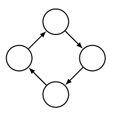
Firstly, let’s get this graph in a usable form. Try writing the graph out as:

[
	(0, empty)
	(1, empty)
	(2, empty)
	(3, empty)
	|
	(4, 0, 1, empty)
	(5, 1, 2, empty)
	(6, 2, 3, empty)
	(7, 3, 0, empty)
]

What does this mean? Well the square brackets [ ... ] surround the entire graph’s structure. Then the nodes are listed, for example; (0, empty) indicates that there is a node which we will identify as node 0 and this node is unlabelled (its label is ‘empty’). After the nodes are listed, there is a divider; |, and then edges are listed. The edge (4, 0, 1, empty) describes an edge from node 0 to node 1 which is also unlabelled.

Save this graph as “cycle.host”.

Try writing this program out in text form:

Main = link!

link(a, b, c, d, e : list)
[
	(n1, a)
	(n2, c)
	(n3, e)
	|
	(e1, n1, n2, b)
	(e2, n2, n3, d)
]
=>
[
	(n1, a)
	(n2, c)
	(n3, e)
	|
	(e1, n1, n2, b)
	(e2, n2, n3, d)
	(e3, n1, n3, empty)
]
interface = 
{
	n1, n2, n3
}
where not edge(1, 3)

and saving it as “transitive_closure.gp2”. The general form of a program in text form is:

Main = [PROGRAM CODE]

[RULE 1]
[RULE 2]
[RULE 3]

And an individual rule is of the form:

[RULENAME]
(
	[VARIABLES]
)
[LEFT HAND SIDE GRAPH]
=>
[RIGHT HAND SIDE GRAPH]
interface = { [INTERFACE] }
[CONDITION]

Where graphs are of the same form as the graph we saw earlier.

So what does our program mean? The only line of the main program is Main = link!. This ! means that the rule link will be applied as long as possible - e.g. it will be applied until it is no longer applicable. Applying the rule link firstly searches for a match for its left hand side; 3 adjacent nodes where there is not an edge from the 1st node to the 3rd node. Then, once a match is found, the left hand side is transformed into the right hand side by inserting an edge from the 1st node to the 3rd node. The ‘interface’ describes which nodes survive; none of the 3 matched nodes n1, n2, n3 are deleted.

Now we can compile our program by calling:

gp2 PATH/TO/transitive_closure.gp2

This will generate c code in the directory “/tmp/gp2”. We can build this generated c code into a program by calling:

make

This will generate a file “/tmp/gp2/gp2run” which is a runnable implementation of our program. We can run this program on our graph by calling:

./gp2run PATH/TO/cycle.host

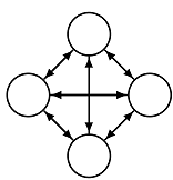
If everything’s gone to plan this will generate a file “/tmp/gp2/gp2.output” which contains this produced graph:

alt text